Theoretical models are only as good as their ability to predict reality. Following our exploration of the theory behind Nonlinear Analysis, this article puts those concepts to the test. Here, we present four comparative case studies where analytical predictions from SeismoStruct and SeismoBuild are benchmarked against full-scale experimental results. From the iconic 4-storey ICONS frame tested at ELSA to a 7-storey shear wall building tested at UCSD, we demonstrate the accuracy and reliability of nonlinear modeling in capturing displacement demands and failure mechanisms in practical engineering scenarios.

In the subsequent sections a series of examples is presented, whereby analytical predictions are compared against measured quantities of the true dynamic behaviour, as measured during experimental tests. In all cases, SeismoStruct was employed for the execution of the nonlinear analyses, however similar results could have been obtained with SeismoBuild, which shares the same analytical engine with SeismoStruct.

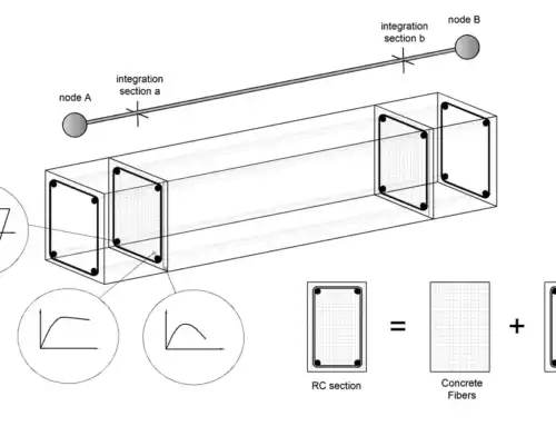
All the structural models employed feature nonlinear characteristics that enable them to correctly identify the structural behaviour and failure mechanisms in the highly-inelastic range. Material inelasticity is represented through fibre modelling with the distributed plasticity approach. Different types of frame elements were employed, e.g. force-based, force-based plastic hinge or displacement-based element types, and geometric nonlinearities are automatically incorporated in the model by the program.

This example describes the modelling of a full-scale, four-storey, 2D bare frame, which was designed essentially for gravity loads and a nominal lateral load of just 8% of its weight (Fig. 1). The reinforcement details attempted to reproduce the construction practices used in southern European countries in the 1950’s and 1960’s. The building was modelled as a plane, three-bay RC frame. The dimensions are indicated in Fig. 2.

The frame was tested at the ELSA laboratory (Joint Research Centre, Ispra) under two subsequent pseudo-dynamic loadings. Further information about the ICONS frame and the tests conducted in ELSA, can be found in Pinto et al. (1999), Carvalho et al. (1999), Pinho and Elnashai (2000) and Varum (2003).

Fig. 1: ICONS frame tested at the ELSA laboratory of Ispra

Fig. 2: Four-storey, three-bay RC frame geometry (elevation and plan views, Carvalho et al. [1999])

The analytical results, obtained with the FE analysis program SeismoStruct, are compared with the experimental results. Two different models were created:

• Model A: Both columns and beams were modelled through 3D force-based inelastic frame elements with 4 integration sections.
• Model B: Both columns and beams were modelled through 3D displacement-based inelastic frame elements.

The masses, proportional to the tributary areas, were applied either (i) as lumped masses at each beam-column joint or (ii) as distributed masses along the beams.
Two artificial records (Acc475 and Acc975, with 475 and 975 year return periods respectively) separated by a 35 sec interval, were run in series for the dynamic time-history analysis. The two input motions are given in Fig. 3 and Fig. 4. The FE model is presented in Fig. 5.

Fig. 3: Artificial acceleration time-history for 475 year return period (Acc-475)

Fig. 4: Artificial acceleration time-history for 975 year return period (Acc-975)

Fig. 5: FE model of ICONS frame in SeismoStruct

The comparison between experimental and analytical results, in terms of total displacement against time is shown in Fig. 6 and Fig. 7. The analysis provided a very good estimate of the structural response throughout the duration of the vibration for both records. It is noted that in the large Acc-975 record, the test was stopped for safety reasons, due to the heavy damage sustained by the building.

Fig. 6: Experimental vs. Analytical results – top displacement vs. time (475yrp)

Fig. 7: Experimental vs. Analytical results – top displacement vs. time (975yrp)

This example case study concerns a prototype building, seven-storey, full-scale RC shear wall frame presented in Fig. 8, tested on the NEES Large High-Performance Outdoor Shake Table at UCSD’s Englekirk Structural Engineering under dynamic conditions (Panagiotou et al. 2006), by applying four subsequent uniaxial ground motions.

Fig. 8: Seven-storey, full-scale RC shear wall building tested at the NEES Large High-Performance Outdoor Shake Table at UCSD’s Englekirk Structural Engineering Center (Martinelli P. and Filippou F.C., 2009)

As depicted in Fig. 8 and Fig. 9, the frame consists of (i) a cantilever web wall, (ii) a flange wall, (iii) a precast segmental pier and (iv) gravity columns. At each floor, the slab is simply supported by the wall and the columns.

Fig. 9: Frame geometry (floor plan view) (Martinelli P. and Filippou F.C., 2009)

Both walls were modelled through 3D force-based inelastic frame elements with 4 integration sections. The number of fibres used in section equilibrium computations was 200. The pinned gravity columns were modelled through truss elements, where the number of fibres used in section equilibrium computations was set to 200. The precast column, since it was designed in order to remain elastic, is modelled through an elastic frame element. Finally, the modelling of the slabs was realized through rigid diaphragms. The masses were computed from the values of weights given by the organizing committee and are assigned in a lumped fashion to each floor node. Finally, the base nodes are fully restrained, so that the anchorage between the structure and the shaking table is modelled.

The applied ground motion is shown in Fig. 10, and the FE model is depicted in Fig. 11:

Fig. 10: Input ground motion

Fig. 11: FE model of the tested 7-storey RC shear wall building in SeismoStruct

The comparison between experimental and analytical results is shown in Fig. 12 and Fig. 13, for both the total displacement and the base shear time-histories. Again, the analysis provided a very good estimate of the structural response for the entire record, even for large drifts and very high levels of inelasticity.

Fig. 12: Experimental vs. Analytical results – top displacement vs. time (EQ4)

Fig. 13: Experimental vs. Analytical results – base shear vs. time (EQ4)

Example 3 presents the nonlinear modelling of a full-scale, three-storey, three-dimensional RC building, which was designed for gravity loads only, according to the 1954-1995 Greek Code. The prototype building was built with the construction practice and materials used in Greece in the early 70’s (non-earthquake resistant construction). It is regular in height but highly irregular in plan (Fig. 14 and Fig. 15). Details on the structural beam member dimensions and reinforcing bars can be found in Fardis and Negro (2006). The prototype building, shown in Fig. 14, was tested at the European Laboratory for Structural Assessment (ELSA) of the Joint Research Centre of Ispra (Italy) under pseudo-dynamic conditions using the Herceg-Novi bi-directional accelerogram registered during the Montenegro 1979 earthquake.

Fig. 14: Full-scale, three-storey prototype building (Fardis & Negro, 2006)

Fig. 15: Plan view of the full-scale, three-storey prototype building (Lanese et al., 2008)

Columns and beams were modelled through 3D displacement-based inelastic frame elements with the number of section fibres set to 200. Applied masses are distributed along columns and beams, while all foundation nodes were considered as fully restrained against rotations and translations. Slabs were modelled by introducing a rigid in-plane diaphragm for each floor level.

Two input acceleration time-histories were used, H-BCR-140 for the X and H-BCR-140 for the Y direction, which are shown in Fig. 16 and Fig. 17. The building FE model is shown in Fig. 18:

Fig. 16: H-BCR140 accelerogram in the X direction

Fig. 17: H-BCR230 accelerogram in the Y direction (b)

Fig. 18: FE model of the building in SeismoStruct

Fig. 19 presents a comparison between experimental and analytical results, in terms of total displacements, which are again in good agreement.

Fig. 19: Experimental vs. Analytical results – displacement vs. time

This is an example that describes the modelling of a prototype building (full-scale, 3D steel moment resisting frame presented in Fig. 20) tested on the world’s largest three-dimensional shaking table located at Miki City, Hyogo Prefecture (Japan) under dynamic conditions, by applying a scaled version of the near-fault motion recorded in Takatori during the 1995 Kobe earthquake. The testing was carried out in the framework of the 2007 Blind Analysis Contest announced by the executive committee of the E-Defense steel building project (NRIESDP, 2007). Additional 3D shaking table tests have been performed consecutively with increasing levels of seismic motion to evaluate the effect of plastic deformation: Takatori scaled to 40% (elastic level), Takatori scaled to 60% (incipient collapse level) and Takatori in full scale (collapse level). Details on the prototype building including geometrical and material characteristics are summarized by Pavan (2008).

The analytical results obtained using a 3-D model developed in SeismoStruct after the test (post-test results), are compared with experimental results. The modelled building is schematically presented in Fig. 21.

Fig. 20: Four-storey 3D steel moment resisting frame (NRIESDP, 2007)

Fig. 21: Four-storey 3D steel frame geometry (frontal and lateral views) (Pavan, 2008)

Two different models of the modelled building were developed:

Model A: In Model A, columns and beams were modelled through 3D force-based inelastic frame elements with 4 integration sections.
Model B: In Model B, columns and beams were modelled through 3D displacement-based inelastic frame elements.

The masses attached to the model were computed from the values of weights given by the organizing committee and were assigned to the beam sections as additional mass. The base nodes were fully restrained, in order to model the anchorage between the structure and the shaking table, and the slabs were modelled as rigid in plane diaphragms for each floor. The analytical model is shown in Fig. 22.

Fig. 22: Four-storey 3D steel frame geometry (3D model) in SeismoStruct

The acceleration time-history applied during the dynamic analysis had three components in the East-West, North-South and Vertical directions. Each time-history consisted of three acceleration records in series separated by a 10 sec interval between them, as shown in Fig. 23, Fig. 24 and Fig. 25.

Fig. 23: Post-test shaking table acceleration time-history (NS component)

Fig. 24: Post-test shaking table acceleration time-history (EW component)

Fig. 25: Experimental Post-test shaking table acceleration time-histories (vertical component)

The analytical and experimental results in terms of maximum relative displacement in the two horizontal directions (North-South and East-West) are shown in Fig. 26, while the results in terms of the maximum storey shear are presented in Fig. 27. Again, in all cases the experimental results are in good agreement with the numerical predictions for both models A and B.

Fig. 26: Experimental vs. Analytical results – maximum relative displacement-floor level

Fig. 27: Experimental vs. Analytical results – maximum storey shear-floor level

This is a case study that presents the modelling of the full-scale, four-storey building, designed according to initial versions of Eurocode 8 and Eurocode 2 and tested at the ELSA laboratory (Joint Research Centre, Ispra). The building was tested with under pseudo-dynamic loading using floor time-histories derived from an accelerogram recorded in the 1976 Friuli earthquake. The building is shown in Fig. 28.

Fig. 28: Four-storey 3D infilled frame tested by Negro et al. (1996)

A 3-D model of the tested building was created in SeismoStruct and consisted of three RC frames (two infilled exterior frames and one bare interior frame) in the North-South direction and three bare RC frames in the South-West direction. The geometric characteristics of the model are presented in Fig. 29 while the building FE model is presented in Fig. 30.

Fig. 29: Four-storey 3D infilled frame geometry (frontal and plan views) (Negro et al., 1996)

Fig. 30: FE model of the tested building created in SeismoStruct

The RC columns and beams were modelled with force-based inelastic frame elements with 4 integration sections, and the sections were subdivided in 200 fibres. Multiple sections were assigned to some beam elements, in order to account for the change in reinforcement between the middle of the beams and their two edges. The infill panels were modelled through a four-node masonry panel element.

The structural mass was modelled as lumped masses, which were then automatically converted to gravity loads by SeismoStruct. The slabs were modelled as rigid diaphragms. All the base nodes were considered fully restrained against rotations and translations.

In Fig. 31 the base shear time-histories, obtained during the test and computed from the analysis, are plotted against time. It is evident that there is excellent agreement between the measured values from the test and the analytical predictions.

Fig. 31: Experimental vs. Analytical results – base shear vs. time

This example describes the modelling of the full-scale reinforced concrete bridge column presented in Fig. 32. The specimen was tested on the NEES Large High-Performance Outdoor Shake Table at UCSD’s Englekirk Structural Engineering Center under dynamic conditions, as part of a blind prediction contest. The geometric characteristics of the column are shown in Fig. 33, while further details can be found in Bianchi et al. (2011). Six uniaxial earthquake ground motions, starting with low-intensity shaking, were increased, so as to bring the pier progressively to near-collapse conditions.

SeismoStruct was employed for the specimen modelling by the winner in the Practitioners category, and was also used by two other teams that received an ‘Award of Excellence’, amongst a total of 41 entries.

Fig. 32: Full-scale reinforced concrete bridge column tested on the NEES Large High-Performance Outdoor Shake Table at UCSD’s Englekirk Structural Engineering Center

Fig. 33: Pier cross section and bridge pier specimen configuration (Bianchi et al., 2011)

The FE model of the pier consisted of a single 3D force-based inelastic frame element, and the number of fibres used in section equilibrium computations was set to 300. The self-mass of the pier along with a lumped mass of 228 ton concentrated at the top of the pier (see Fig. 33) were taken into consideration. The FE model is presented in Fig. 34.

Fig. 34: FE model of the bridge column in SeismoStruct

During the nonlinear dynamic analysis of the model, an acceleration time series consisting of six ground motion records (EQ1 to EQ6) in series separated by 10 sec intervals were generated. The time series used in the analysis are shown in Fig. 35, Fig. 36 and Fig. 37.

Fig. 35: Input ground motion (EQ1 and EQ2)

Fig. 36: Input ground motion (EQ3 and EQ4)

Fig. 37: Input ground motion (EQ5 and EQ6)

The comparison between numerical and experimental results for the top displacement is shown in Fig. 38, Fig. 39 and Fig. 40 for EQ1, EQ3 and EQ5 respectively. The plots with the comparison for the base shear are shown in Fig. 41, Fig. 42 and Fig. 43 for EQ1, EQ3 and EQ5 respectively. Numerical and experimental results are generally in good agreement, even in the highly inelastic range.

Fig. 38: Experimental vs. Analytical results – top displacement vs. time (EQ1)

Fig. 39: Experimental vs. Analytical results – top displacement vs. time (EQ3)

Fig. 40: Experimental vs. Analytical results – top displacement vs. time (EQ5)

Fig. 41: Experimental vs. Analytical results – base shear vs. time (EQ1)

Fig. 42: Experimental vs. Analytical results – base shear vs. time (EQ3)

Fig. 43: Experimental vs. Analytical results – base shear vs. time (EQ5)

Example 7 presents the modelling of two geometrically identical one-storey, three-dimensional RC frame structures (see Fig. 44), which were designed for low and high ductility levels, according to EC8 provisions. In each structure the slab does not cover the entire span, whereas nine large, additional masses are placed on top of it in a non-symmetrical configuration. A schematic plan of the aforementioned model is presented in Fig. 45. Each specimen (i.e. model A and model B, depending on the different steel reinforcement detailing) was tested under dynamic conditions on the LNEC-3D shaking table of Lisbon (Portugal) as part of a Blind Prediction Contest organized at the 15th World Conference on Earthquake Engineering (15WCEE), by applying four input ground motions of increasing intensity levels in each horizontal direction.

SeismoStruct was employed by the winning team, selected amongst a total of 38 participating entries. The numerical results obtained by analysis of the building model developed in SeismoStruct are compared with the experimental results obtained during the testing of the specimens.

Fig. 44: One-storey, three dimensional RC frame structures tested on the LNEC-3D shaking table of Lisbon (Portugal) during the 15WCEE (LNEC team, 2012)

Fig. 45: Plan view of the prototype model with the localization of the masses (LNEC team, 2012)

For the creation of the building FE model (see Fig. 46) columns and beams were modelled through 3D inelastic force-based frame elements with 3÷5 integration sections, depending on the element configuration. The number of fibres used in section equilibrium computations was set to 200.

The additional masses on top of the slab were applied in a lumped fashion, considering also the rotational inertia. The additional masses are connected to each other and to the adjacent beams through the use of elastic frame elements with the section properties of the slab.

Two time-histories were used for the nonlinear analysis of the model, one for each loading direction (NS and EW). Each time-history consists of four acceleration time-series (EQ1, EQ2, EQ3 and EQ4) separated by 10 sec intervals. The entire time-history used for loading the model along the East-West direction is shown in Fig. 47, while the time- history used for the North-South direction is shown in Fig. 48.

Fig. 46: FE model of the structure in SeismoStruct

Fig. 47: Input ground motion in the X direction (East-West component)

Fig. 48: Input ground motion in the Y direction (North-South component)

The comparison between experimental and analytical top displacement for Model A under the EQ3 record in the East-West and North-South directions is shown in Fig. 49 and Fig. 50. Equivalent results are presented in Fig. 51 and Fig. 52 for Model B. In spite of apparent differences, numerical and experimental results seem to agree well for both models.

Fig. 49: Experimental vs. Analytical results – top displacement vs. time (EQ3_REF)_Comp X

Fig. 50: Experimental vs. Analytical results – top displacement vs. time (EQ3_REF)_Comp Y

The comparison between experimental and analytical results for model B is shown hereafter:

Fig. 51: Experimental vs. Analytical results – top displacement vs. time (EQ3_REF)_Comp X

Fig. 52: Experimental vs. Analytical results – top displacement vs. time (EQ3_REF)_Comp Y

The examples presented in this post demonstrate that the gap between experimental observation and analytical prediction can be effectively bridged when nonlinear analysis is grounded in sound physical modelling and transparent numerical assumptions. Across a broad spectrum of structural systems—ranging from simple frames to highly irregular three-dimensional buildings and bridge components—the analytical simulations reproduced measured responses with a high degree of consistency, even under severe inelastic demand. This is particularly evident in large-scale shake-table experiments and blind prediction exercises, where prior calibration to test outcomes was not possible.

From a practical standpoint, the close agreement between analytical and experimental results supports the use of nonlinear dynamic analysis as a credible decision-making tool in performance-based assessment and design. When applied within a consistent modelling philosophy and validated against experimental evidence, such analyses provide engineers with confidence not only in numerical results, but also in the structural interpretations derived from them.

Ultimately, experimental testing and analytical simulation form a continuous feedback loop: experiments validate modelling strategies, while analytical tools extend experimental insight to real-world structures that cannot be tested directly. It is within this balance—between theoretical rigor, numerical robustness, and practical engineering judgement—that nonlinear analysis proves its true value in engineering practice.

• Bianchi F., Sousa R., Pinho R. 2011. Blind prediction of a full-scale RC bridge column tested under dynamic conditions. Proceedings of 3rd International Conference on Computational Methods in Structural Dynamics and Earthquake Engineering (COMPDYN 2011). Paper no. 294, Corfu, Greece.
• Carvalho E.C., Coelho E., Campos-Costa A. 1999. Preparation of the Full-Scale Tests on Reinforced Concrete Frames. Characteristics of the Test Specimens, Materials and Testing Conditions. ICONS Report, Innovative Seismic Design Concepts for New and Existing Structures. European TMR Network, LNEC.
• Fardis, M.N. and Negro P. 2006. SPEAR – Seismic performance assessment and rehabilitation of existing buildings. Proceedings of the International Workshop on the SPEAR Project, Ispra, Italy.
• Lanese I., Nascimbene R., Pavese A., Pinho R. 2008. Numerical simulations of an infilled 3D frame in support of a shaking-table testing campaign. Proceedings of the RELUIS Conference on Assessment and Mitigation of Seismic Vulnerability of Existing Reinforced Concrete Structures, Rome, Italy.
• LNEC team [2012] “Blind Test Challenge Report”, Report, LNEC (National Laboratory for Civil Engineering), Portugal.
• Martinelli P. and Filippou F.C. 2009. Simulation of the Shaking Table Test of a Seven-Storey Shear Wall Building, Earthquake Engineering and Structural Dynamics, 38, No. 5, : 587-607.
• Negro P., Pinto A.V., Verzeletti G., Magonette G.E. [1996] PsD Test on a Four-Storey R/C Building Designed According to Eurocodes, Journal of Structural Engineering – ASCE 122(11) 1409-1417.
• National Research Institute for Earth Science and Disaster Prevention 2007. Hyogo Earthquake Engineering Research Center. Blind Analysis Contest. URL: www.bosai.go.jp/hyogo/ehyogo/index.html
• Panagiotou M., Restrepo J.I. and Englekirk R.E. 2006. Experimental seismic response of a full scale reinforced concrete wall building, Proceedings of the First European Conference on Earthquake Engineering and Seismology, Geneva, Switzerland, Paper no. 201.
• Pavan A. 2008. Blind Prediction of a Full-Scale 3D Steel Frame Tested under Dynamic Conditions, MSc Dissertation, ROSE School, Pavia, Italy.
• Pinho, R. and Elnashai, A.S. 2000. Dynamic collapse testing of a full-scale four storey RC frame. ISET Journal of Earthquake Technology Paper No. 406; 37(4) : 143-164.
• Pinto A., Verzeletti G., Molina F.J., Varum H., Pinho R., Coelho E. 1999. Pseudo-Dynamic Tests on Non-Seismic Resisting RC Frames (Bare and Selective Retrofit Frames). EUR Report, Joint Research Centre, Ispra, Italy.
• Seismosoft .2026. SeismoBuild 2026 – A computer program for static and dynamic nonlinear analysis of framed structures. Available from URL: www.seismosoft.com
• Seismosoft .2026. SeismoStruct 2026 – A computer program for static and dynamic nonlinear analysis of framed structures. Available from URL: www.seismosoft.com
• Varum, H. 2003. Seismic Assessment, Strengthening and Repair of Existing Buildings, PhD Thesis, Department of Civil Engineering, University of Aveiro