In the assessment of existing structures, traditional linear elastic analysis often falls short, failing to capture the true behavior of buildings under seismic loads—especially when damage and inelasticity occur. This article serves as the first part of our deep dive into Nonlinear Structural Analysis, focusing on the fundamental theory and numerical formulation behind these advanced methods. For real-world validation of these theories, we also created Case Studies in Nonlinear Analysis that put these theoretical concepts to the test.

From the onset of structural analysis, engineers have employed linear elastic methods, implicitly assuming small deformations, limited damage to structural members, and an approximately elastic response of all structural components. Even in today’s practice, elastic methods are still widely used for the design of new structures. This is not unreasonable, considering that in new structures engineers are able to select the strength and stiffness characteristics of the structural components so as to achieve a reasonable distribution of inelasticity among different members, without large concentrations of inelastic deformations at particular, more vulnerable locations of the building.

This, together with careful detailing of the members (e.g. closely spaced stirrups in RC members or diagonal reinforcement where needed) and the adoption of a uniform behaviour factor (q-factor) that accounts for the inelastic response (implicitly assuming that inelasticity is approximately evenly distributed throughout the structure), provides an efficient and reasonably accurate framework for the design of new structures with a high level of reliability.

However, the true structural behaviour is inevitably nonlinear, and buildings designed and constructed prior to the introduction of modern seismic design codes still constitute a large percentage of the existing building stock. These structures were designed primarily for gravity loads, without specific provisions to resist seismic actions in a manner consistent with current practice. As a result, they often exhibit irregular arrangements of structural members, with uneven distributions of strength, stiffness, and mass in plan or elevation, which adversely affect their behaviour under earthquake loading (e.g. soft storeys, short columns, coupling beams between large shear walls, indirect beam supports, etc.).

Consequently, the use of elastic analysis procedures for existing buildings may lead to significant inaccuracies in estimating both the force and deformation demands of structural components. Moreover, in most cases this approximation results in an underestimation of displacement demands at locations where inelastic deformations tend to concentrate—typically the most vulnerable regions under seismic loading.

As a result, the engineering community over the last three decades has started to study the use of nonlinear structural analysis, especially under loading, which is expected to cause large inelastic deformations, such as earthquake loading.

Even today, the seismic design of buildings is predominantly based on linear elastic analysis, despite the general acknowledgment that such an approach lacks accuracy and may lead to significant underestimations of both force and deformation demands when compared with inelastic analysis. Linear analysis requires substantially less computational effort and fewer resources than nonlinear analysis. Until relatively recently (mid-1990s), the computational power available was insufficient to support the widespread adoption of nonlinear analysis in structural design and assessment. Moreover, the design methodologies currently in use were largely developed several decades ago, when nonlinear procedures were not widely applied, owing not only to limited computational resources but also to insufficient understanding of nonlinear structural behaviour within the engineering community.

Nevertheless, true structural behaviour is inherently nonlinear, characterized by a non-proportional relationship between displacements and applied loads, particularly in the presence of large deformations or material nonlinearities. This is especially relevant in seismic structural analysis, since most structures are not designed to remain elastic during maximum seismic events due to economic considerations and uncertainties in predicting seismic demand. Instead, they are expected to undergo significant inelastic deformations under strong ground motions. Consequently, structural analyses should, in principle, be treated as potentially nonlinear. The fundamental objective is to exploit structural ductility and post-elastic strength in order to satisfy prescribed performance criteria while minimizing capital investment.

Nonlinear analysis methods enable the estimation of structural response beyond the elastic range, explicitly accounting for strength and stiffness degradation associated with inelastic material behaviour and large displacements. As such, they provide a highly efficient and accurate analytical framework for capturing realistic structural behaviour, with fewer simplifying assumptions and more direct, performance-oriented design criteria.

Supported by recent advances in computing technologies and the growing availability of experimental and analytical data, the use of nonlinear structural analysis has become increasingly widespread. It now plays a central role in the assessment of existing buildings and is increasingly adopted in the design of new structures, either directly through performance-based design methodologies or indirectly through the evaluation of structures designed using advanced elastic approaches.

The first comprehensive guidelines for the application of nonlinear analysis were published in the mid-1990s, notably FEMA-273: NEHRP Guidelines for the Seismic Rehabilitation of Buildings (FEMA, 1997) and ATC-40: Seismic Evaluation and Retrofit of Concrete Buildings (ATC, 1996). Subsequent improvements were introduced in FEMA-440: Improvement of Nonlinear Static Seismic Analysis Procedures (FEMA, 2005) and FEMA-P440A: Effects of Strength and Stiffness Degradation on Seismic Response (FEMA, 2009a). Nonlinear analysis methodologies have since been incorporated into modern seismic assessment frameworks, including ASCE-41: Seismic Rehabilitation of Existing Buildings (ASCE, 2023), Eurocode 8 – Part 3 (EN 1998-3, 2004), and national codes in several countries, such as Italy, Greece, and Turkey. Furthermore, nonlinear analysis concepts have been widely employed in seismic risk assessment methodologies, most notably in HAZUS (Kircher et al., 1997a; Kircher et al., 1997b; FEMA, 2009b).

Nonlinear analysis is commonly applied in structural earthquake engineering practice in the following cases:

1. Evaluation and retrofit of existing buildings. Most existing buildings do not comply with modern seismic detailing requirements, making elastic analysis inadequate for reliable assessment and retrofit design. Nonlinear analysis enables a more realistic estimation of structural capacity and deformation demands, often allowing less conservative interventions and reduced retrofit costs. Consequently, seismic assessment of existing buildings has been a primary driver for the adoption of nonlinear analysis, particularly within performance-based assessment frameworks (Antoniou 2025a, Antoniou 2025b, Antoniou 2023)
2. Verification and performance assessment of new buildings. Nonlinear analysis is increasingly used to supplement elastic design by providing a more accurate prediction of structural response. Modern performance-based methodologies, such as ATC-58 (Applied Technology Council, 2009), employ nonlinear dynamic analysis to relate structural demands to explicit damage, loss, and performance metrics for both new and existing buildings.
3. Design of buildings with non-conventional systems or materials. The use of advanced materials and systems—such as fibre-reinforced polymers, shape-memory alloys, supplemental damping, and base isolation—often lies outside the scope of prescriptive code provisions. In such cases, nonlinear (static or dynamic) analysis is required to capture the full hysteretic behaviour and interaction of these systems.
4. Design of tall buildings in high seismicity regions. Tall buildings frequently employ nonstandard seismic-force-resisting systems and performance objectives exceeding minimum code requirements. As a result, nonlinear dynamic analysis is routinely mandated by specialized guidelines for performance-based seismic design of high-rise buildings.
5. Performance-based design with owner-defined objectives. Performance-based engineering allows owners to specify target performance levels that can be analytically evaluated and optimized through life-cycle cost considerations. Nonlinear analysis provides the accuracy and flexibility needed to reliably assess such customized performance objectives.
6. Seismic risk assessment. Nonlinear analysis is increasingly used in seismic risk and loss assessment frameworks, such as HAZUS, to develop building-specific fragility functions and improve the reliability of damage and loss predictions.

Although nonlinear analysis is undoubtedly superior in terms of the accuracy of structural response predictions, this improvement does not come without cost. The computational demands of nonlinear analysis are substantial, particularly for large-scale models subjected to dynamic loading.

Moreover, whereas linear analysis accounts primarily for the mass and stiffness distribution of structural members, nonlinear analysis requires explicit consideration of member strength, inelastic behaviour, and deformation- and force-based limit states. This necessitates the definition of component models capable of representing force–deformation relationships at both the element and system levels, including the effects of large deformations. Such modelling requires detailed knowledge of the structural configuration, as well as experienced engineers and additional effort to achieve an adequate level of modelling fidelity.

In addition, the results of nonlinear analyses can be highly sensitive to assumed input parameters and modelling choices. Without sufficient expertise in nonlinear assessment methods, engineers may draw misleading conclusions regarding structural performance. Generally, it is advisable to have clear expectations about those portions of the structure that are expected to undergo inelastic deformations, so as to use the analyses to confirm the locations of inelastic deformations.
Finally, unlike linear elastic procedures—which are well established and have been extensively validated over several decades—nonlinear inelastic analysis techniques are relatively recent and continue to evolve. Consequently, their effective application requires ongoing professional development, including continuous training, the acquisition of advanced analytical skills, and familiarity with rapidly evolving computational tools.

In linear structural analysis things are relatively simple and straightforward. Every element has linear cross-section properties EA, EI2, EI3, GJ and constant stiffness. The stiffnesses of all the elements are summed up to form the global stiffness matrix [K] of the building, which is also constant, and [K] is inverted once for the solution of the well-known equation P=[K]·u and the calculation of the nodal displacements for the different load cases. What is more, because the stiffness matrix is always positive-definite and the member strengths are considered unlimited, there will always be a mathematical solution to the problem.

Because in nonlinear analysis the structural stiffness matrix is no longer constant, but rather it is updated at every step, and because there is a strength limit in all or most of the structural members, the solution of the nonlinear equations becomes a much more complicated task. In the next sections the main points of the theoretical background of nonlinear analysis will be presented briefly.

Despite the maturity of the finite element (FE) method, the seismic assessment of buildings is performed primarily with linear finite elements (e.g. beams or rods), while two- and three-dimensional FE are very rarely utilized. Further, apart from modelling the frame members with beam-column elements, the numerical model of a structure should also be able to adequately capture the response of other structural components, such as infill panels, that may considerably affect the overall capacity.

The modelling of the mechanical properties of the structural members is a complex and wide-ranging subject. In linear analysis, it is sufficient to assume that the material remains linear and elastic, i.e. that the deformation process is fully reversible and the stress is a unique function of strain. However, such a simplified assumption is appropriate only within a limited range, and is gradually being replaced by more realistic approaches.

The primary source of nonlinearities in low and medium-rise building structures is material inelasticity and plastic yielding in the locations of damage. In larger high-rise buildings, while material inelasticity still plays an important role, large deformations relative to the frame element’s chord (known as P-Delta effects), and geometric nonlinearities become equally important and should be taken into account.

Material nonlinearities occur when the stress-strain or force-displacement law is not linear, or when material properties change with the applied loads. Contrary to linear analysis procedures, where the material stresses are always proportional to the corresponding strains and a fully elastic behaviour is assumed, in nonlinear analysis the material behaviour depends on current deformation state and possibly past history of the deformation. In order to estimate the stress from the strain of a particular location of the structure, complete expressions for the uniaxial stress-strain relationship of the material should be provided, including hysteretic rules for unloading and reloading.

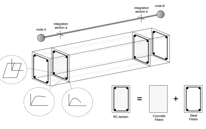
The source of such inelasticity is defined at the sectional level, through the creation of a fibre model for the section. A fibre section consists in the subdivision of the area in n smaller areas, each of which is attributed a material stress-strain relationship, i.e. reinforcing steel and concrete, confined and unconfined. After defining the material laws of every material of the section, and calculating the stresses at the fibres, the sectional moment-curvature state of beam-column elements is then obtained through the integration of the nonlinear uniaxial stress-strain response of the individual fibres. The discretisation of a typical reinforced concrete cross-section is depicted in Fig. 1.

Estimating the inelastic response of the structural member requires the integration of the stresses calculated at appropriately selected integration cross-sections along the member (called Gauss Sections a and b, in Fig. 1). Finally, the global nonlinearity of the frame is then obtained by the assembly of the contributions in stiffness and strength of the structural components.

Fig 1: Discretisation of a typical reinforced concrete cross-section

Geometric nonlinearities involve nonlinearities in kinematic quantities, and occur due to large displacements, large rotations and large independent deformations relative to the frame element’s chord (also known as P-Delta effects).

The effect of geometric nonlinearities on the response of structures can range from negligible, in cases where large deformations are not expected, to extreme, in large and slender structures. In the general case, geometric nonlinearities must be modelled as they can ultimately lead to loss of lateral resistance, ratcheting (a gradual build-up of residual deformations under cyclic loading), and dynamic instability. Large lateral deflections magnify the internal force and moment demands, causing a decrease in the effective lateral stiffness. With the increase of internal forces, a smaller proportion of the structure’s capacity remains available to sustain lateral loads, leading to a reduction in the effective lateral strength.

For the numerical simulation of geometric nonlinearities and the inclusion of its effects in the analysis, the most advanced formulation is a total co-rotational formulation [Correia and Virtuoso, 2006], which is based on an exact description of the kinematic transformations associated with large displacements and three-dimensional rotations of the beam-column member. This leads to the correct definition of the element’s independent deformations and forces, as well as to the natural definition of the effects of geometrical non-linearities on the stiffness matrix.

In the local chord system of the beam-column element, six basic displacement degrees-of-freedom (θ2(A), θ3(A), θ2(B), θ3(B), Δ, θT) and corresponding element internal forces (M2(A), M3(A), M2(B), M3(B), F, MT) are defined, as shown in Fig. 2.

Fig. 2: Local chord system of a beam-column element

Once the governing equations of geometrically nonlinear structural analysis and the discretization of those equations by finite element methods is completed, a procedure is required for the solution of these equations. Nonlinear problems in mechanics are solved with incremental algorithms through a process that is considerably more complex than that used in common linear elastic analysis solvers.

All solution procedures of practical importance are strongly rooted in the idea of gradually advancing the solution by continuation, that is to follow the equilibrium response of the structure as the control and state parameters vary by small amounts. Various algorithms exist for handling such problems, but a common feature is that continuation is a multilevel process that involves a hierarchical breakdown into incremental steps, and iterative steps. The level of incrementation is always present in nonlinear solution procedures. To advance the solution, the entire loading stage is broken down into incremental steps, also called increments or steps. The incremental solution methods are then divided into two broad categories: (1) Purely incremental methods, also called predictor-only methods, and (2) Corrective methods, also called predictor-corrector or incremental-iterative methods.

In purely incremental methods the iteration level is missing. In corrective methods a predictor step is followed by one or more iteration steps. The set of iterations is called the corrective phase. Its purpose is to eliminate or reduce the so called drifting error, which is a serious problem of purely incremental methods. For this reason the corrective methods have become the standard for the solution of the nonlinear equations in all modern finite element packages.
Solutions accepted after each increment following a corrective phase are often of interest to users because they represent approximations to equilibrium states until the final loading state. They are therefore saved as they are computed. On the other hand, intermediate results of the iterative process are rarely of interest, since the solutions are not equilibrated and constitute an intermediate step until the next equilibrated solution. Hence, most programs discard them.

The use of increments may seem at first sight unnecessary if one is interested primarily in the final solution. But breaking up a stage into increments may serve different purposes: (i) The presence of path-dependent effects in nonlinear analysis problems severely restricts increment sizes because of history-tracing constraints. For example, in plasticity analysis stress states must not be allowed to stray too far outside the yield surface. (ii) The engineer can acquire a better insight into structural behaviour by studying the response plot toward the final solution, which in many cases can provide more useful information than simply the structural state at the end. It is noted that in several cases failures and critical points occur before the stage end. (iii) The breakdown of the entire loading stage can lead to more stable solutions and avoid convergence problems.

The basic method for the solution of nonlinear equations in the majority of finite element programs is the load-control Newton-Raphson (NR) algorithm and variations of it. The Newton-Raphson method, in its simplest form, is a numerical method for finding the roots of a function f(x). Since the method is iterative, a trial guess is made at x=xn. Evaluating the function at xn, we find that f (xn)≠0, i.e. it is not a root. If f’(xn) is the tangent of the function at xn, the equation of the tangent passing through xn, is:

With the aid of equation (1), we can obtain a second trial solution at xn+1:

where xn+1 is the point where the tangent intersects axis X. If f (xn+1) ≈ 0, then we have located the root, otherwise we proceed finding a new trial solution at xn+2, until convergence to the correct solution has been reached within an acceptable convergence limit. The method is schematically shown in Fig. 3.

Fig. 3: Application of the Newton-Raphson (NR) method for finding the roots of a function f(x)

In structural mechanics the Newton-Raphson (NR) method is extended, so that to accommodate the solution of a system of nonlinear equations, as described by the general equation of equilibrium:

Because of the nonlinear nature of the problem, the stiffness matrix K is a function of the deformation vector u and is constantly updated at each iteration, and hence the system of Eq. (3) cannot be solved directly, and should follow an incremental-iterative solution procedure that is called the Newton-Raphson method.

Fig. 4: The Newton-Raphson (NR) method in nonlinear structural analysis

The incremental-iterative Newton-Raphson method is schematically shown in Fig. 4. The iterative procedure follows the conventional scheme, whereby the internal forces corresponding to a displacement increment are computed and convergence is checked. If no convergence is achieved, then the out-of-balance forces (difference between applied load vector and equilibrated internal forces) are applied to the structure, and the new displacement increment is computed. Such loop proceeds until convergence has been achieved or the maximum number of iterations has been reached. Load-displacement plots, such as those of Fig. 4 are exact for one SDOF systems. For larger MDOF systems, they describe only schematically the structural response and the gradual convergence to the solution of the system of equations.

The full Newton-Raphson method provides a quadratic rate of convergence, meaning that it requires a small number of iterations to reach the solution. However, recalculating and inverting the stiffness matrix at every iteration requires increased computing resources. Hence, a common alternative is to recalculate and invert the stiffness matrix only at the first iteration and use it for all the corrective iterations. This approach is known as modified Newton-Raphson and is shown in Fig. 5.

The employment of Newton-Raphson (NR), modified Newton-Raphson (mNR) or NR-mNR hybrid solution procedures may lead to fairly flexible solution algorithm. It is clear that the computational savings in the formation, assembly and reduction of the stiffness matrix during the iterative process can be significant when using the mNR instead of the NR procedures. However, more iterations are often required with the mNR, thus leading, in some cases, to excessive computational effort. For this reason, the hybrid approach, whereby the stiffness matrix is updated only in the first few iterations of a load increment, does usually lead to an optimum scenario.

For further discussion and clarifications on the algorithms described above, readers are strongly advised to refer to available literature, such as the work by Cook et al. [1988], Crisfield [1991], Zienkiewicz and Taylor [1991], Bathe [1996] and Felippa [2002], to name but a few.

Fig. 5: The Modified Newton-Raphson (mNR) method in nonlinear structural analysis

In iterative-incremental solution algorithms, the iterative process at each step is continued, until ‘convergence is achieved’, that is the value of a norm of the out-of-balanced forces or the unbalanced deformations of the structure become smaller than given convergence criteria that have been specified by the user at the beginning of the analysis.

There are two distinct categories of convergence criteria in nonlinear analysis:

1. displacement/rotation-based criteria
2. force/moment-based criteria.

Two additional convergence check schemes may arise from the combination of the distinct criteria above:

3. Displacement/Rotation AND Force/Moment based scheme, where it is considered that the solution has been reached, when both the deformation and the force based criteria have been achieved
4. Displacement/Rotation OR Force/Moment based scheme, where convergence is achieved, when either the deformation or the force based criteria has been achieved.

Usually, the displacement/rotation criterion consists in verifying, for each individual degree-of-freedom of the structure, that the current iterative displacement/rotation is less or equal than a user-specified tolerance. In other words, if and when all values of displacement or rotation that result from the application of the iterative (out-of-balance) load vector are less or equal to the pre-defined displacement/rotation tolerance factors, then the solution is deemed as having converged. This concept can be mathematically expressed in the following manner:

where,

• δdi is the iterative displacement at translational degree of freedom i
• δθj is the iterative rotation at rotational degree of freedom j
• nd is the number of translational degrees of freedom
• nθ is the number of rotational degrees of freedom
• dtol is the displacement tolerance, in the employed by the analysis length unit
• θtol is the rotation tolerance, in rad (dimensionless)

The force/moment criterion, on the other hand, comprises the calculation of the Euclidean norm of the iterative out-of-balance load vector, and subsequent comparison to a user-defined tolerance factor. It is therefore a global convergence check (convergence is not checked for every individual degree-of-freedom as is done for the displacement/rotation case) that provides an indication of the overall state of convergence of the solution, and which can be mathematically described in the following manner:

where,

• Gnorm is the Euclidean norm of iterative out-of-balance load vector
• Gi is the iterative out-of-balance load at degree-of-freedom i
• VREF is the reference ‘tolerance’ value for forces (translational DOFs) and moments (rotational DOFs). Typically, different values are assumed for VREF
• for the translational and the rotational DOFs
• n is the number of the degrees-of-freedom

It is noted that, contrary to linear analysis, where a solution, even if it is unreasonable and unrealistic, can always be found, in the case of nonlinear analysis, the achievement of convergence and the calculation of the solution is not always guaranteed. This is due to purely ‘technical’ reasons (e.g. a beam cannot withstand the applied vertical loads, fails and a solution cannot be found), but also numerical reasons (e.g. if the solution procedure cannot accommodate large load increments, or sudden redistribution of forces, after the failure of a load-carrying member).

For this reason, in nonlinear analysis the maximum number of iterations is always specified, so that to avoid searching for a solution infinitely. If the maximum number of iterations is reached and convergence has not been achieved, the analysis is either stopped, or in more advanced software packages the load step is subdivided in smaller increments, in order to achieve better convergence conditions.

In addition to the convergence verification scheme described above, at the end of an iterative step three other solution checks may be carried out; numerical instability, solution divergence and iteration prediction. These criteria, all of a force/moment nature, serve the purpose of avoiding the computation of useless equilibrium iterations in cases where it is apparent that convergence will not be reached, thus minimising the duration of the analysis.

Numerical instability: The possibility of the solution becoming numerically unstable is checked at every iteration by comparing the Euclidean norm of out-of-balance loads, Gnorm, with a pre-defined maximum tolerance several orders of magnitude larger than the applied load vector (e.g. 1.0E+20). If Gnorm exceeds this tolerance, then the solution is assumed as being numerically unstable and iterations within the current increment are interrupted.
Solution divergence: Divergence of the solution is checked by comparing the value of Gnorm obtained in the current iteration with that obtained in the previous one. If Gnorm has increased, then it is assumed that the solution is diverging from a possible solution and iterations within the current increment are interrupted.

Iteration prediction: Finally, a logarithmic convergence rate check is also carried out, so as to try to predict the number of iterations required for convergence to be achieved. If this calculated number of iterations is larger than the maximum number of iterations specified by the user, then it is assumed that the solution will not achieve convergence and iterations within the current increment are interrupted.

Within the context of all modern Codes, two types of nonlinear analysis procedures are proposed for structural assessment: (i) the Nonlinear Static Procedure (NSP), also is called pushover analysis. (ii) ) the Nonlinear Dynamic Procedure (NDP), that is, the nonlinear dynamic time-history analysis.

According to ASCE 41, Section 7.4.3.1 (ASCE, 2023), in the Nonlinear Static Procedure, a mathematical model directly incorporating the nonlinear load-deformation characteristics of individual components of the building shall be subjected to monotonically increasing lateral loads representing inertia forces in an earthquake, until a target displacement is exceeded. The main objective of the method is to assess the capacity of the structure, considering both the deformability and strength of all structural members.

The lateral loads are gradually applied until the displacement of a selected ‘Control Node’, typically located at the centre of mass of the top storey of the building, reaches the so-called ‘Target Displacement’, which represents an approximation of the displacement demand under earthquake ground motion. The demand parameters for the structural components at the target displacement are then compared against the respective acceptance criteria for the desired performance state. System level demand parameters, such as story drifts and base shear forces, may also be checked.

Although the nonlinear static procedure is generally a much more reliable approach for characterizing the performance of a structure than linear procedures, it is still not exact and cannot accurately account for changes in the dynamic response as the structure degrades in stiffness; nor can it account for higher mode effects in multi-degree-of-freedom (MDOF) systems. Hence, the NSP is applicable to low-rise, regular buildings, where the response is dominated by the fundamental sway mode of vibration. It is less suitable, however, for taller, slender, or irregular buildings, where multiple vibration modes affect the behaviour.

According to ASCE 41-23, Section 7.4.4.1 (ASCE, 2023), in the Nonlinear Dynamic Procedure, a mathematical model directly incorporating the nonlinear load-deformation characteristics of individual components of the building shall be subjected to earthquake shaking represented by ground motion acceleration histories to obtain forces and displacements. The objective of the method is to assess the capacity of the structure, considering both the deformability, the strength and the hysteretic behaviour of all structural members that are subjected to the specified earthquake ground motion.

The direct integration of the equations of motion is accomplished using certain integration algorithms, such as the numerically dissipative α-integration algorithm (Hilber et al., 1977) or a special case of the former, the well-known Newmark scheme (Newmark, 1959). The modelling of seismic action is achieved by introducing acceleration loading curves (accelerograms) at the supports. In addition, dynamic analysis may also be employed for modelling of pulse loading cases (e.g. blast, impact, etc.), in which case instead of acceleration time-histories at the supports, force pulse functions of any given shape (rectangular, triangular, parabolic, and so on), can be employed to describe the transient loading applied to the appropriate nodes.

The NDP constitutes a sophisticated approach to examining the inelastic demands produced on a structure by a specific suite of ground motion acceleration histories. As with the NSP, the results of the NDP can be directly compared with test data on the behaviour of representative structural components to identify the structure’s probable performance, when subjected to a specific ground motion.

As nonlinear dynamic analysis involves fewer assumptions than the nonlinear static procedure, it is subject to fewer limitations than nonlinear static procedure. It automatically accounts for higher-mode effects and shifts in inertial load patterns as structural softening occurs. In addition, for a given earthquake record, this approach directly solves for the maximum global displacement demand produced by the earthquake on the structure, eliminating the need to estimate this demand based on general relationships.

Despite these advantages, the NDP requires considerable judgment and experience to perform, and should only be used when the engineer is thoroughly familiar with nonlinear dynamic analysis techniques and limitations. The analyses can be highly sensitive to small changes in assumptions with regard to either the character of the ground motion record used in the analysis or the nonlinear stiffness behaviour of the elements. For instance, two ground motion records enveloped by the same response spectrum can produce radically different results with regard to the distribution and amount of inelasticity predicted in the structure. Further, due to the inherent variability in earthquake ground motions, dynamic analyses for multiple ground motions are necessary to calculate an upper bound for the values of the demand parameters for a given earthquake scenario.

By more realistically representing the underlying structural mechanics, nonlinear static analysis and especially nonlinear dynamic analysis, reduce uncertainty in demand predictions, as compared to the linear methods of analysis. However, even with nonlinear dynamic analyses, it is practically impossible to always calculate accurately the demand parameters for the different structural members. Hence, very often there are discrepancies between the analytical predictions of the response parameters and their actual values during a seismic event. These discrepancies are usually largest for structural deformation and acceleration controlled quantities, and lower in force-controlled components, where internal forces are bounded by the strength of yielding members.

Since no numerical representation of the components response is exact, one of the sources of inaccuracy is the limitations related to the analytical capabilities of the selected software package itself, with which the analysis is to be carried out. Obviously, any analytical formulation that describes the hysteretic behaviour of materials, sections or members has limitations that restrain its ability to represent the structural response in a very precise manner, especially in the highly inelastic range, where the lateral stiffness is significantly reduced and the response is very sensitive to small changes of the loading. Analysts should be well aware of these limitations prior to the execution of the analyses, so that to avoid modelling strategies that magnify the possible errors and affect considerably the analytical predictions.

Nonetheless, continued advances in computational tools and modelling techniques have progressively reduced software-related inaccuracies, especially for ordinary structures with components exhibiting predictable behaviour that can be represented with reasonable accuracy. In such cases, the dominant sources of uncertainty are typically human- and data-related, namely: (i) variability and uncertainty in measured physical properties such as material characteristics, geometry, and detailing, and (ii) incomplete or imperfect representation of the actual structural behaviour in the analytical model. When combined with seismic hazard uncertainties—such as variability in ground motion intensity, frequency content, and duration—these factors can lead to substantial divergence between analytical predictions and true structural response during strong earthquakes.

In light of the above, analysts should explicitly recognize and account for the various sources of uncertainty inherent in structural evaluation. Where possible, these uncertainties should be quantified and reflected in acceptance criteria through the appropriate selection of safety or modification factors. The chosen values should be consistent with the level of confidence in both the structural information and the analytical model. For example, assessment frameworks assign different values to the knowledge factor (ASCE 41-23) or the confidence factor (Eurocode 8, Part 3), with more conservative values adopted when the available information on the structure is limited.

One means of assessing the accuracy achievable by analytical procedures is through blind prediction exercises. In such studies, engineers are asked to predict the response of a structure—whose true behaviour will be determined through experimental testing—without prior knowledge of the measured results, using state-of-the-art analytical tools. This approach provides an unbiased evaluation of predictive capability, as prior knowledge of the response cannot be used to calibrate or refine the simulations.

In recent years, numerous blind prediction exercises have been conducted, ranging from single structural components and subassemblies to large-scale, full structural systems. In many cases, teams of analysts were invited to predict the response of structures tested on shake tables, based solely on information regarding structural design and the characteristics of the imposed ground motions.

Results from these exercises have consistently shown significant scatter among predicted responses, often leading to poor agreement with measured behaviour, including nonlinear response mechanisms and failure modes. This indicates that many predictions remain unreliable in practice. Moreover, drawing definitive conclusions from such studies is challenging, as discrepancies may arise from multiple sources, including inconsistent characterization of input parameters, inaccuracies in material modelling, insufficient mesh refinement, or limitations of the adopted nonlinear modelling approaches.

Nevertheless, blind prediction exercises are invaluable for identifying and evaluating the sources of variability between analytical predictions and experimental observations, as well as for distinguishing analytical procedures that perform consistently better—or worse—than others. Careful examination of past blind prediction studies can therefore provide critical insight into the strengths and limitations of nonlinear analysis methods and contribute to the systematic improvement of their reliability.

Theoretical formulations and numerical models are only as valuable as their ability to predict real structural behavior. Now that we have established how the nonlinear methods work, the critical question remains: Do they match reality?

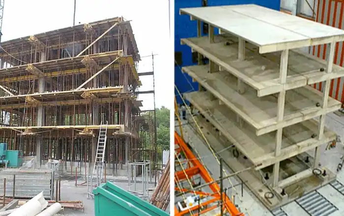
In the second part of this series, we put these theories to the test. We benchmark the analytical predictions of SeismoStruct and SeismoBuild against full-scale experimental results, including the famous ICONS frame tested at ELSA and a 7-storey shear wall building tested at UCSD.

Continue reading: Nonlinear Structural Analysis in Engineering Practice – Case Studies

• Antoniou 2025a. Why Linear Procedures are not suitable for the Seismic Assessment and Retrofit of Existing RC Buildings Available from URL: https://seismosoft.com/linear-procedures-suitable-seismic-assessment-retrofit-existing-buildings/
• Antoniou, S. 2025b. Linear vs. nonlinear procedures for the seismic assessment and retrofit of existing RC buildings. In Proceedings of the 10th International Conference on Computational Methods in Structural Dynamics and Earthquake Engineering (COMPDYN 2025) (Paper C 27254). Rhodes Island, Greece (Available at URL: https://2025.compdyn.org/proceedings/pdf/27254.pdf).
• Antoniou, S. Seismic Retrofit of Existing Reinforced Concrete Buildings, 1st Edition. John Wiley & Sons Ltd, 2023.
• American Society of Civil Engineers. Seismic Evaluation and Retrofit of Existing Buildings, ASCE/SEI 41-23. Reston, Virginia, 2023.
• [ATC] Applied Technology Council, 1996. Seismic Evaluation and Retrofit of Concrete Buildings, ATC-40 Report, Applied Technology Council, Redwood City, California.
• [ATC] Applied Technology Council, 2009. Guidelines for seismic performance assessment of buildings, ATC 58, 50 % Draft Report, Applied Technology Council, Redwood City, CA.
• Bathe K.J. 1996. Finite Element Procedures in Engineering Analysis, 2nd Edition, Prentice Hall.
• Clough R.W., Johnston S.B. 1966. Effect of Stiffness Degradation on Earthquake Ductility Requirements Proceedings, Second Japan National Conference on Earthquake Engineering 1966: 227-232.
• Cook R.D., Malkus D.S., Plesha M.E. 1989. Concepts and Applications of Finite Elements Analysis. John Wiley & Sons.
• Correia A.A., Virtuoso F.B.E. 2006. Nonlinear Analysis of Space Frames, Proceedings of the Third European Conference on Computational Mechanics: Solids, Structures and Coupled Problems in Engineering, Mota Soares et al. (Eds.), Lisbon, Portugal.
• Crisfield M.A. 1991. Non-linear Finite Element Analysis of Solids and Structures, John Wiley & Sons.
• EN 1998-3 [2004]: Eurocode 8: Design of structures for earthquake resistance -Part 3: Assessment and retrofitting of buildings.
• Felippa C.A. 2001. Nonlinear Finite Element Methods, Lecture Notes, Centre for Aerospace Structure, College of Engineering, University of Colorado, USA.
• [FEMA] Federal Emergency Management Agency. 1997. NEHRP Guidelines for the Seismic Rehabilitation of Buildings, FEMA 273 Report, prepared by the Applied Technology Council and the Building Seismic Safety Council for the Federal Emergency Management Agency, Washington, D.C.
• [FEMA] Federal Emergency Management Agency. 2005. Improvement of Nonlinear Static Seismic Analysis Procedures, FEMA 440 Report, prepared by the Applied Technology Council for the Federal Emergency Management Agency, Washington, D.C.
• [FEMA] Federal Emergency Management Agency. 2009a. Effects of Strength and Stiffness Degradation on Seismic Response, FEMA P-440A Report, prepared by the Applied Technology Council for the Federal Emergency Management Agency, Washington, D.C.
• [FEMA] Federal Emergency Management Agency. 2009b. HAZUS®-MH MR5 Advanced Engineering Building Module (AEBM) Technical and User’s Manual, prepared by the National Institute of Buildings Sciences for the Federal Emergency Management Agency, Washington, D.C.
• Hilber H.M., Hughes T.J.R., Taylor R.L. 1977. Improved numerical dissipation for time integration algorithms in structural dynamics. Earthquake Engineering and Structural Dynamics 5( 3) : 283-292.
• Giberson, M.F. 1967. The Response of Nonlinear Multi-Story Structures subjected to Earthquake Excitation, Doctoral Dissertation, California Institute of Technology, Pasadena, CA., May 1967 : 232
• Kircher, C. A., Nassar, A. A., Kustu, O., and Holmes, W. T. 1997a. Development of Building Damage Functions for Earthquake Loss Estimation. Earthquake Spectra 13 (4), : 663-682.
• Kircher, C. A., Reitherman, R. K., Whitman, R. V., and Arnold, C. 1997b. Estimation of Earthquake Losses to Buildings. Earthquake Spectra 13 (4) : 703-720.
• Mari A., Scordelis A. 1984. Nonlinear geometric material and time dependent analysis of three dimensional reinforced and prestressed concrete frames, SESM Report 82-12. Department of Civil Engineering, University of California, Berkeley.
• Neuenhofer A., Filippou F.C. 1997. Evaluation of nonlinear frame finite-element models. Journal of Structural Engineering 123(7) : 958-966.
• Newmark N.M. 1959. A method of computation for structural dynamics. Journal of the Engineering Mechanics Division, ASCE 85( EM3) : 67-94.
• [NIST] National Institute of Standards and Technology. 2010. Nonlinear Structural Analysis for Seismic Design, A Guide for Practicing Engineers, GCR 10-917-5, prepared by the NEHRP Consultants Joint Venture, a partnership of the Applied Technology Council and the Consortium of Universities for Research in Earthquake Engineering, for the National Institute of Standards and Technology, Gaithersburg, Maryland.
• [PEER] Pacific Earthquake Engineering Research Centre. 2010. Tall Buildings Initiative: Guidelines for Performance-Based Seismic Design of Tall Buildings, PEER Report 2010/05, Pacific Earthquake Engineering Research Center, Berkeley, California.
• PEER/ATC .2010. Modeling and acceptance criteria for seismic design and analysis of tall buildings, PEER/ATC 72-1 Report, Applied Technology Council, Redwood City, CA, October 2010.
• Willford, M., Whittaker, A., and Klemencic, R. 2008. Recommendations for the seismic design of high-rise buildings, Council on Tall Buildings and Urban Habitat, Illinois Institute of Technology, Chicago, IL.
• Seismosoft .2026. SeismoBuild 2026 – A computer program for static and dynamic nonlinear analysis of framed structures. Available from URL: www.seismosoft.com
• Seismosoft .2026. SeismoStruct 2026 – A computer program for static and dynamic nonlinear analysis of framed structures. Available from URL: www.seismosoft.com
• Scott M.H., Fenves G.L. 2006. Plastic hinge integration methods for force-based beam–column elements. ASCE Journal of Structural Engineering 132( 2) : 244-252.
• Spacone E., Ciampi V., Filippou F.C. 1996. Mixed formulation of nonlinear beam finite element. Computers & Structures 58( 1) : 71-83.
• Zienkiewicz O.C., Taylor R.L. 1991. The Finite Element Method, 4th Edition, McGraw Hill.